Recently, the Machine Learning community has become more focused on finding invertible transformations. One of the benefits of invertible transformations is that the change of variable formula holds:
$$p_X(x) = p_Z(z) \left | \frac{dz}{dx} \right|, \quad z = f(x),$$
which admits the optimization of a complicated likelihood $p_X(\cdot)$ via a simple, tractable one: $p_Z(\cdot)$. Glow introduced invertible $1 \times 1$ convolutions and i-ResNet introduced invertible residual connections.
Our work aims to invert the convolution operation1 itself. In other words, we want to be able to find the inverse convolution, sometimes referred to as a deconvolution. We introduce three methods: i) emerging convolutions for invertible zero-padded convolutions, ii) invertible periodic convolutions, and iii) stable and flexible $1 \times 1$ convolutions. For details, check out paper or code.
Standard convolutions
To understand how, let’s first study a deep learning convolution. We will assume our kernel $\mathbf{w}$ and input $\mathbf{x}$ are both single channel with height 3 and width 3 pixels. Also, we will assume 1 pixel wide zero padding. It turns out, this convolution (depicted left), can be expressed as a matrix multiplication (right):
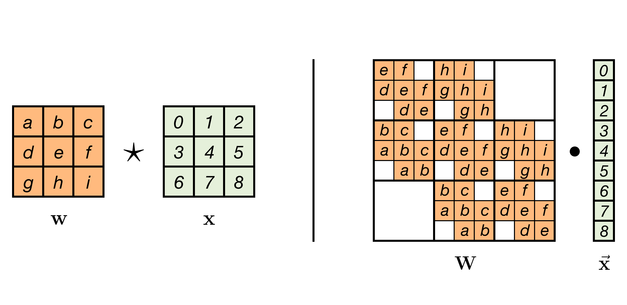
A 1-channel convolution as matrix multiplication
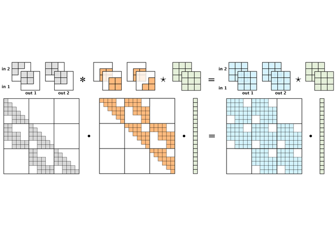
Going further, we can even visualize a multi-channel convolution. For clarity, we omit the value descriptions inside the filter. Let’s visualize a 2-channel convolution:
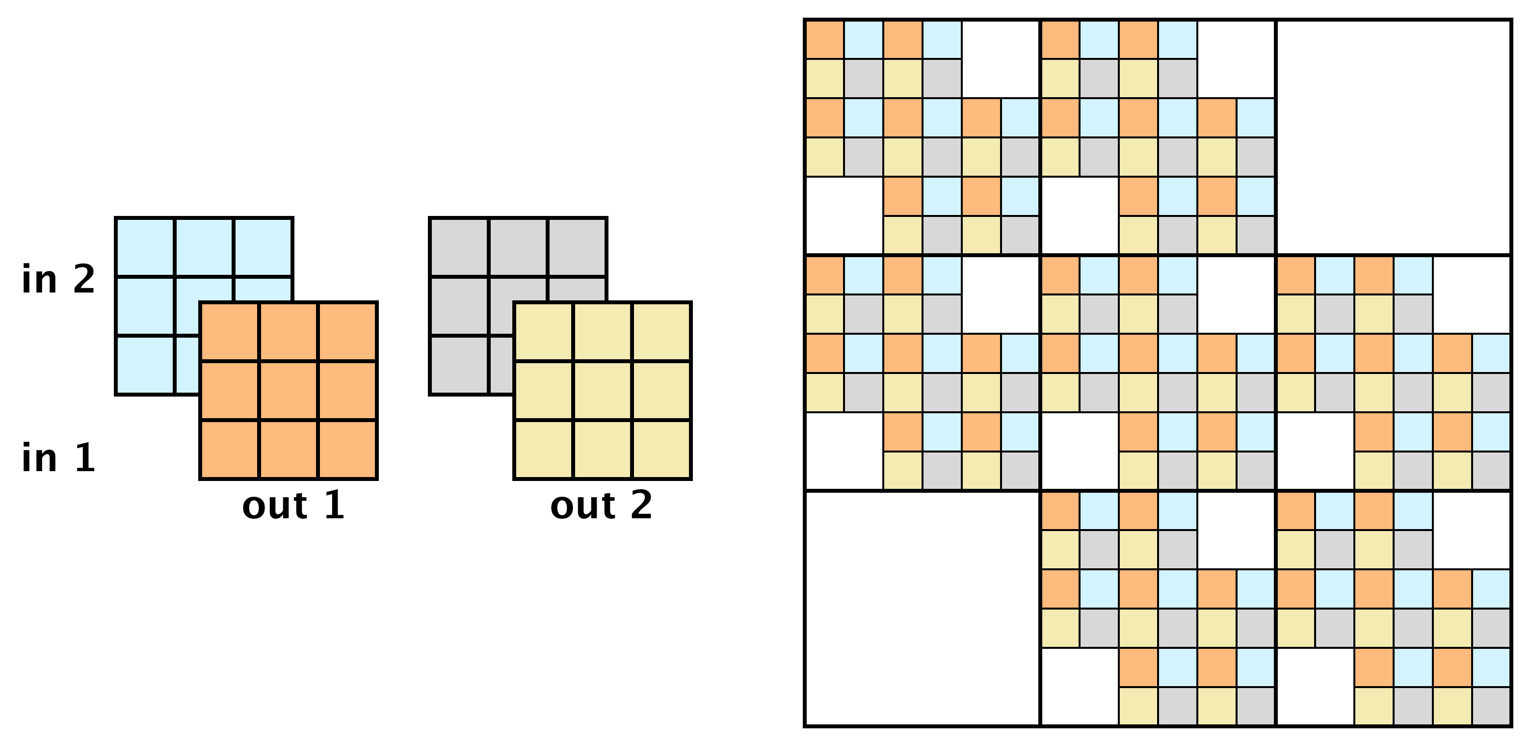
A 2-channel convolution as matrix multiplication
In this figure, the kernel and equivalent matrix are shown without the input. Implicitly, a vector ordering on the input $x$ was chosen to visualize this matrix. It is not very important what this ordering is, as it only determines the order in which the parameter values appear in the matrix.
Now that we have expressed everything as linear algebra, it seems we have solved the problem and we can find the inverse. However, for images of larger size, this matrix would grow quite quickly: It has dimensions $h w c \times h w c$, where $h$ is height, $w$ is width, and $c$ is number of channels. Therefore, even though inverting this matrix directly is technically possible, the growth of the matrix makes this practically infeasible.
Autoregressive Convolutions
Convolution kernels can be masked in a very particular way, such that the equivalent matrix is triangular. As a consequence, it is straightforward to compute the Jacobian determinant and the inverse for this operation. In essence, we have traded complexity for a convolution that is easy to invert:
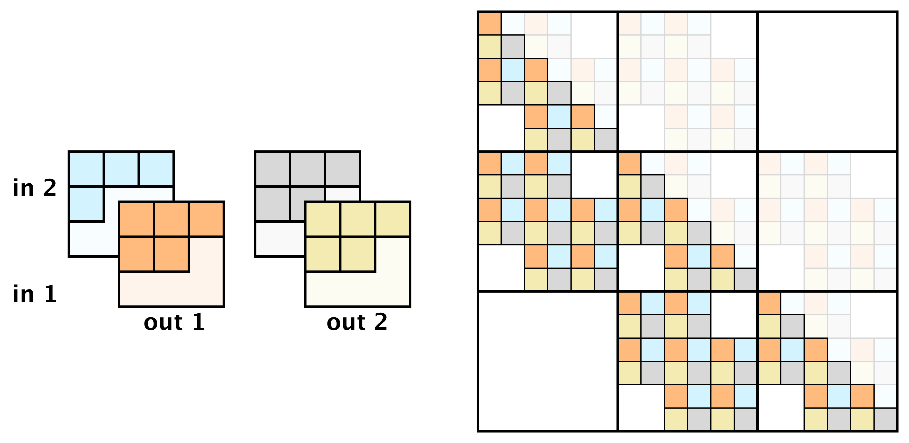
A 2-channel autoregressive convolution as matrix multiplication
Even though the autoregressive convolution is easily inverted, it suffers from limited flexibility: in this case, it is blind to pixels below.
Emerging Convolutions
Now we are all set to create an invertible convolution. The main idea is to combine multiple autoregressive convolutions, with specifically designed masks. As a result, the emerging receptive field is identical to that of a standard convolution: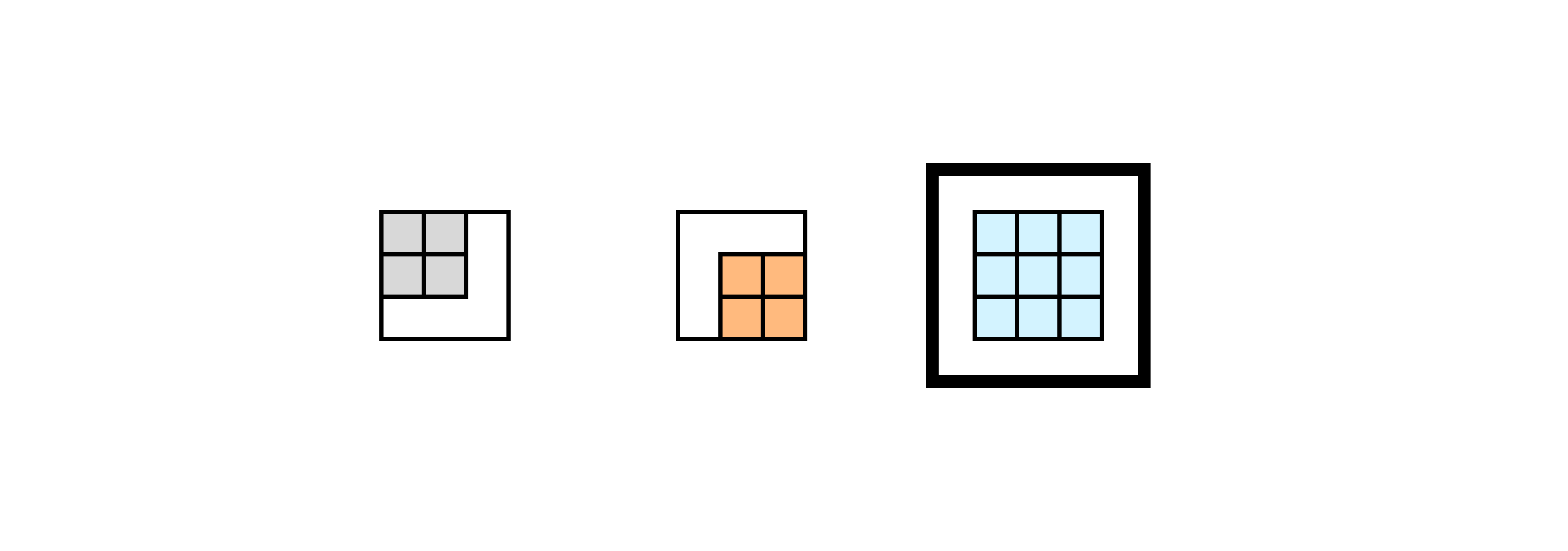
Applying two autoregressive convolutions (left) results in a convolution with a receptive field identical to standard convolutions (right)
This allows one to learn an invertible convolution from a factorization of two masked convolutions. Mathematically, this can be viewed as applying a convolution with filter $k_1$ and then with $k_2$, or as a single convolution2 with filter $k = k_2 * {k_1}$:
$$k_2 \star (k_1 \star f) = (k_2 * {k_1}) \star f.$$
Invertible Periodic Convolutions
Alternative to using factored convolutions, we may also leverage the convolution theorem, which is connected with the Fourier transform. As a consequence, our convolutions will be circular. This can be useful when data is periodic around edges, or if the pixels contain roughly the same values. For the exact details please refer to the paper. In short: the feature maps and kernels are transformed to the frequency domain using the Fourier transform. In the frequency domain, the equivalent matrix of the convolution is a block matrix, and the convolution can be computed as:
$$\hat{\mathbf{z}}_{:,uv} = \hat{\mathbf{W}}_{uv} , \hat{\mathbf{x}}_{:,uv},$$ where the notation $\hat{,}$ denotes a tensor is in the frequency domain, by applying the fourier transform. The inverse is obtained by simply inverting $\hat{\mathbf{W}}_{uv}$. $$\hat{\mathbf{z}}_{:,uv} = \hat{\mathbf{W}}_{uv}^{-1} , \hat{\mathbf{x}}_{:,uv},$$
Although it may seem like we have not gained anything, the matrices $\hat{\mathbf{W}}_{uv}$ are actually independent and small. Instead of a naïve inverse, which would have cost $\mathcal{O}(h^3 w^3 c^3)$, inverting this method has computational cost of $\mathcal{O}(hw c^3)$, which can even be parallelized across the dimensions $w$ and $h$.
Stable 1 $\times$ 1 QR convolutions
In addition to the invertible $d \times d$ convolutions, we also introduce a stable and flexible parametrization of the 1 $\times$ 1 convolution, that uses the QR decomposition. Although any square matrix has a PLU parametrization (as proposed in Glow), it is difficult to train the permutation matrix P using gradient descent. Instead, we introduce a QR parametrization, that can be trained straightforwardly. The inverse is then simply obtained by applying a 1 $\times$ 1 convolution using the kernel $R^{-1} Q^\text{T}$.
Conclusion
In summary, we have introduced three generative flows: i) $d \times d$ emerging convolutions as invertible standard zero-padded convolutions, ii) $d \times d$ periodic convolutions for periodic data or data with minimal boundary variation, and iii) stable and flexible $1 \times 1$ convolutions using a QR parametrization. If you want to know more, check out paper or code.
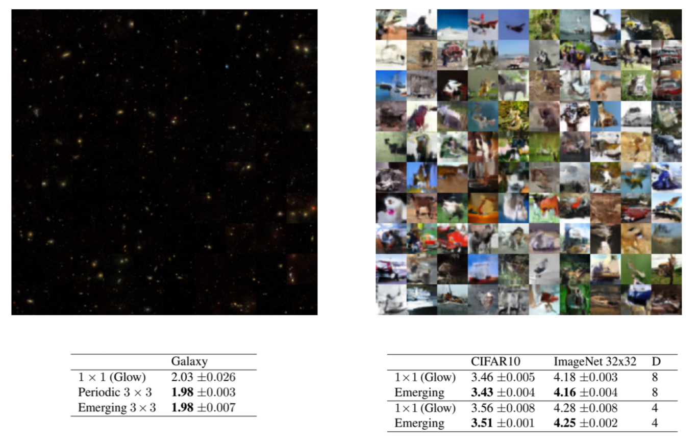
Left: samples from a flow using periodic convolutions trained on galaxy images. Right: samples from a flow using emerging convolutions trained on CIFAR10. Bottom: Performance in bits per dimension, i.e. negative log$_2$-likelihood (lower is better)
References
Hoogeboom, E., Van Den Berg, R. & Welling, M.. (2019). Emerging Convolutions for Generative Normalizing Flows. Proceedings of the 36th International Conference on Machine Learning, in PMLR 97:2771-2780
Kingma, D. P., Dhariwal, P.. Glow: Generative Flow with Invertible 1x1 Convolutions. Advances in Neural Information Processing Systems 31.
Behrmann, J., Grathwohl, W., Chen, R.T.Q., Duvenaud, D. & Jacobsen, J.. (2019). Invertible Residual Networks. Proceedings of the 36th International Conference on Machine Learning, in PMLR 97:573-582