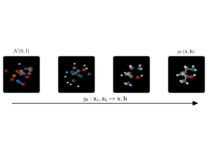
A quick motivation. A nice application of our E(n) Normalizing Flow (E-NF) is the simultaneous generation of molecule features and 3D positions. However the method also aimed to be general-purpose and can be used for other data as well. You can think about point-cloud data, or even better point-cloud data with some features on the point (like a temperature). E-NFs can learn a distribution over data like that. After learning such a distribution, we can sample new points that resemble the data, if successful ;).
The aim of this blog post is to guide you through some of the techniques we used to make E(n) Equivariant Flows (paper). I really liked working on this project because it nicely brought together several topics in literature. For some of these, there are related previous projects that I was a part of. To give an overview, this blog is on:
- Normalizing Flows
- Continuous Time Normalizing Flows
- E(n) Equivariant GNNs
- Argmax Flows
- And then finally tying everything together for E(n) Normalizing Flows.
These sections are aimed to be as much stand-alone as possible, although they are of course connected. Also, this write-up is intended to be an intro, and is should not be seen as comprehensive or complete. For more details and a more thorough exposition, please see the paper. I hope you will enjoy it :)
1. Normalizing Flows and the change of variables formula
Main takeaway Normalizing flows are invertible functions. We generally name the flow $f$ and its inverse $g = f^{-1}$, which you can also name “flow”. The flow contains neural networks and can be learned from data. Flows allow exact likelihood computation via the change of variables formula. The difficult part is often finding a nice (learnable) function that is invertible. After training, flows can be used to generate data. Confession: To this date I am still unsure why they are called “normalizing”. Some people say because they map to a normal distribution, others say because they re-normalize the distribution after the map.
A Generative Model. A generative model is often defined using a simple distribution $p_Z$ and a learnable function $g: \mathbf{z} \mapsto \mathbf{x}$. For the simple distribution we desire something that we can sample from, and we call this the base distribution. This distribution lives in some other space than the data itself, called the latent space. We will name a variable of this space $\mathbf{z}$ and without much imagination we will pick the base distribution over $\mathbf{z}$ to be Gaussian, so $p_Z(\mathbf{z}) = \mathcal{N}(\mathbf{z} | 0, 1)$.
Next we want to initialize some neural network to model $g: \mathbf{z} \mapsto \mathbf{x}$. However, without any constraints on $g$, in practice we can only sample from this model. Sampling works like this: First sample $\mathbf{z} \sim p_Z$ (using torch.randn() for instance) and then compute $\mathbf{x} = g(\mathbf{z})$. This procedure implies a distribution $p_X(\mathbf{x})$. Okay so sampling is easy. The difficulty is optimizing such a model. Given a new datapoint $\mathbf{x}$ it is extremely difficult to compute the likelihood $p_X(\mathbf{x})$.
Let’s see an example in 1D:
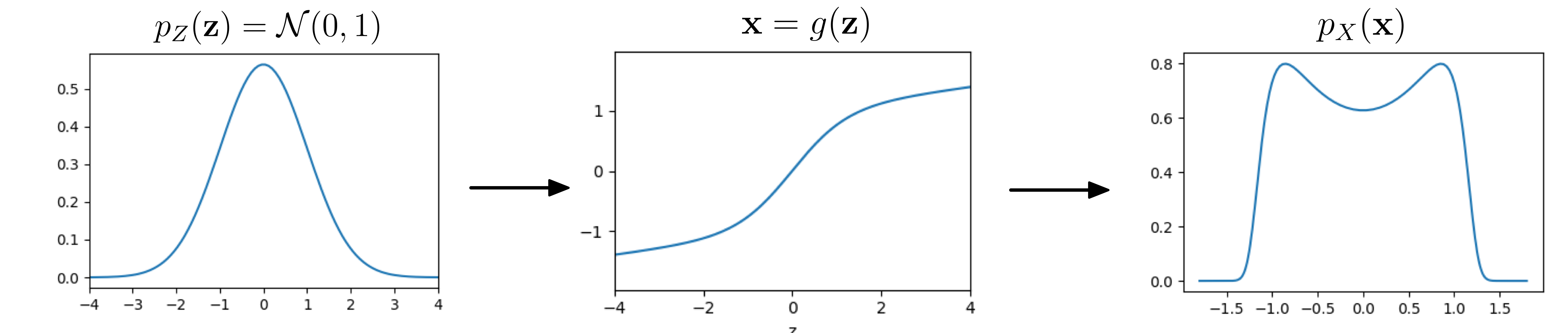
A simple distribution $p_Z$ is fed through a function $\mathbf{x} = g(\mathbf{z})$ to give $p_X$
Magic! By composing a simple distribution with a somewhat complicated function $g$, we have created a distribution with two peaks from a unimodal Gaussian. To build some intuition, think about the following: If the derivative of $g$ is high, will the resulting density in $p_X$ at that point become lower or higher? To reiterate the point of the previous paragraph: it is generally difficult to compute $p_X$. Huh? But how did we do it in this example then? Secretly, the example has been handcrafted so that $g$ is invertible. It turns out, $g$ is already a flow…
Normalizing Flows.
To compute $p_X(\mathbf{x})$, Normalizing Flows (Rezende & Mohamed 2015, Dinh et al. 2016) come to the rescue, they restrict $g$ to be invertible. As a result we can utilize the change of variables formula. In 1 dimension it reads:
$$p_X(\mathbf{x}) = p_Z(g^{-1}(\mathbf{x})) \left| g’(g^{-1}(\mathbf{x})) \right|^{-1}.$$
with $g’$ as derivative. In more dimensions the formula is:
$$p_X(\mathbf{x}) = p_Z(g^{-1}(\mathbf{x})) \left | \det J_g(g^{-1}(\mathbf{x})) \right|^{-1}.$$
That is interesting, we find the likelihood of a point $\mathbf{x}$ by inverting $g$ and going back to the corresponding latent point $\mathbf{z}$. Also we are using the Jacobian determinant of the function at some point. Funny is that there is a lot of inverses $g^{-1}$ in the formula. It turns out we need the inverse more than $g$ itself! For that reason we often learn the inverse directly and call this $f = g^{-1}$. This is possible because if $f$ is invertible, then $g$ is too. It’s only changing the perspective a little. After writing everything in terms of $f$ the change-of-variables formula looks like this:
$$p_X(\mathbf{x}) = p_Z(\mathbf{z}) \left | \det J_f(\mathbf{x}) \right|, \quad \mathbf{z} = f(\mathbf{x}).$$
Okay, what does this formula mean? First of all it’s good to recall that we are interested in learning a complex model distribution, something that can capture all the intricate dependencies of our data. We call this model distribution $p_X$. Ideally, we want a sample $\mathbf{x} \sim p_X$ to look like a sample from the data, after we’ve trained our model. So this formula tells us that given a datapoint $\mathbf{x}$, we should transform it using $\mathbf{z} = f(\mathbf{x})$ and compute two things: $p_Z(\mathbf{z})$ and the Jacobian determinant $\det J_f(\mathbf{x})$. Multiply these things and we get the likelihood $p_X(\mathbf{x})$.
Going back to the example, we can look at $f$, which is the inverse of $g$:
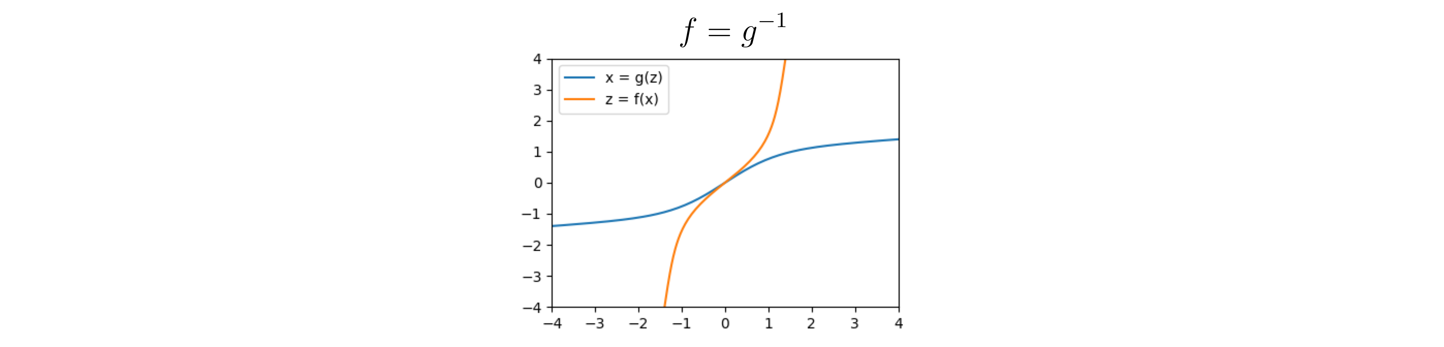
The inverse of $g$
Using this function $f$ and given a data distribution, we can now do some inference, that is we can compute the likelihood of datapoints under our model, and observe how it compares to the true data distribution:
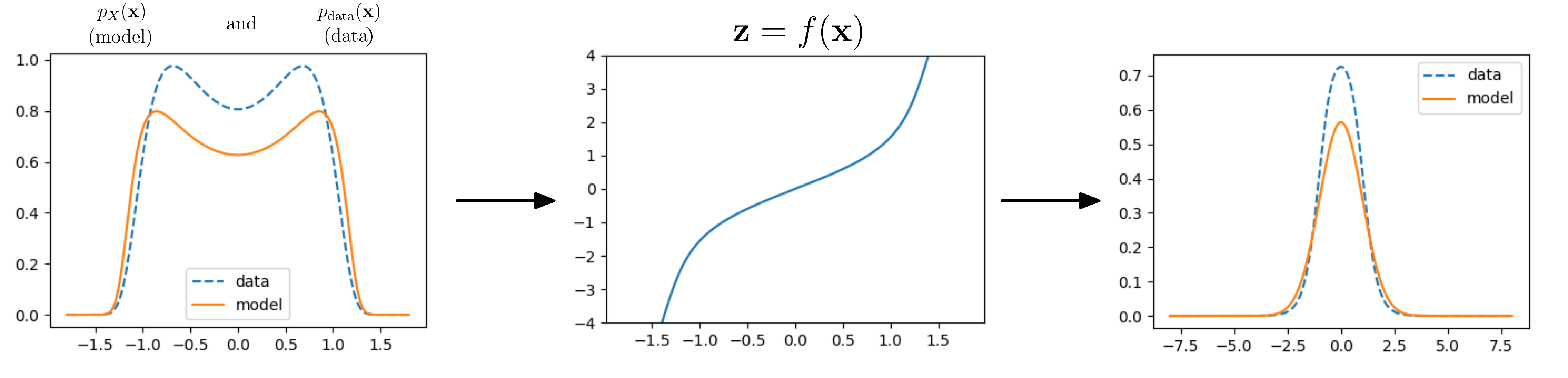
Data and model distribution. $f$ tries to shape data into a Gaussian.
Awesome! We now have a method to learn a model distribution $p_X$ that fits to samples from some dataset. In practice training looks like this: We get a datapoint $\mathbf{x}$. We compute the corresponding latent point $\mathbf{z} = f(\mathbf{x})$ and then compute $p_Z(\mathbf{z})$ and $|\det J_f(\mathbf{x})|$. We then multiply these together to get the model likelihood of the datapoint $\mathbf{x}$. The function $f$ is optimized to maximize $p_X(\mathbf{x})$. Sampling goes like this: Sample $\mathbf{z} \sim p_Z$ (using torch.randn()) and then compute $\mathbf{x} = g(\mathbf{z}) = f^{-1}(\mathbf{z})$. A small detail: In higher dimension log-space generally works a lot better for optimization and in that case the change-of-variable looks like: $$\log p_X(x) = \log p_Z(z) + \log \left | \det J_f(x) \right|, \quad z = f(x).$$
This is the intro to normalizing flows. There is already a much better blogpost written by Jakub here, but I made you read through my version first :). Be sure to check it out for more details!
2. Continuous-time Normalizing Flows
Main takeaway Continuous-time Normalizing Flows come from a beautiful insight: solutions to ordinary differential equations (ODEs) are almost always invertible (under some very mild constraints). This is awesome, the reason: ODEs are a very easy way to build a flow, which we call continuous-time flows. And we only need to put mild constraints on the neural network $\phi$ inside the ODE, mainly some differentiability. For an illustration of a 1 dimensional continuous-time flow see below:
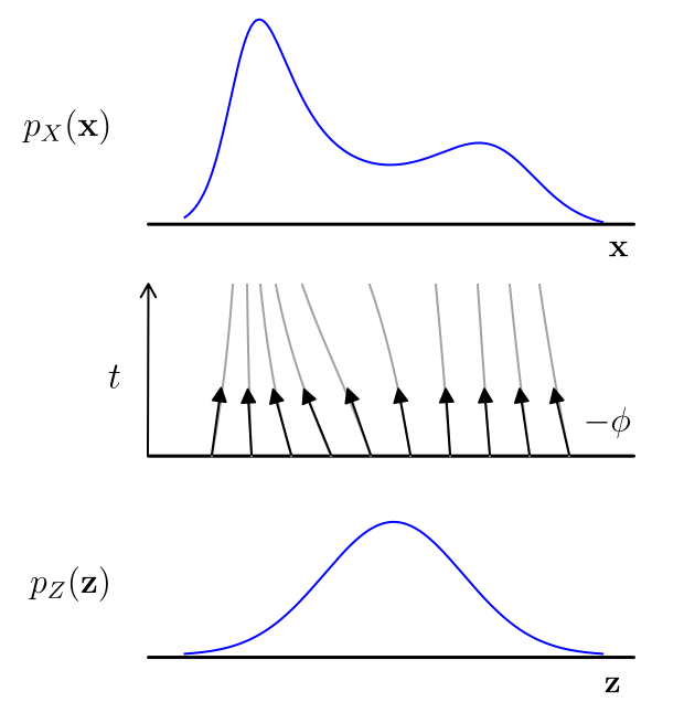
A continuous-time flow generates a more complicated 1D distribution from a Gaussian. This visualization was inspired by the figure from Grathwohl et al. (2018)
The Transformation
An ODE can be formulated like this:
$$\mathbf{z} = \mathbf{x} + \int_0^1 \phi(\mathbf{x}(t)) dt$$
where $\phi$ models the first order derivative with respect to time. Only time is not really time, it’s more a conceptual thing to think about the ODE. We will not go into detail into how to solve such a thing, but rest assured that there is a beautiful python package written by Chen et al. (2018) to do so called torchdiffeq. In code solving the above really amounts to calling z = odeint(self.phi, x, [0, 1]). To me, this simplicity is magical. To connect this to the previous section, we say that $f$ gives the solution to the ODE, so that $\mathbf{z} = f(\mathbf{x})$.
As claimed before, the inverse to this equation exists. It is:
$$\mathbf{x} = \mathbf{z} + \int_1^0 \phi(\mathbf{x}(t)) dt$$
and is solved by calling x = odeint(self.phi, z, [1, 0]). Again, we take this entire transform and call it $g= f^{-1}$ from the previous section. Since it’s invertible, we can use it as a flow: a continuous-time normalizing flow (Chen et al 2017, Chen et al. 2018)
Continuous-time change-of-variables. Just having an invertible function is not enough. We also need to find $J_f(\mathbf{x})$ to compute the log-likelihood of a datapoint $\mathbf{x}$. We can find that the continuous time change-of-variables is written as:
$$\log p_X(\mathbf{x}) = \log p_Z(\mathbf{z}) + \int_0^1 \mathrm{Tr }\, J _{\phi}(\mathbf{x}(t)) dt$$
It turns out that $\log \det J_f = \int_0^1 \mathrm{Tr }\, J _{\phi}(\mathbf{x}(t)) dt$. So the change of variables formula is written as another ODE. By the way, this can also be solved using odeint. Without giving a formal proof, there is a nice identity via the matrix logarithm that you can use to see the connection between log determinant and the trace. The identity is: $\log \det J = \mathrm{Tr }\, \log J$. Observe that this second $\log$ is the matrix logarithm. Imagine taking a small step (like in Euler’s method) for small $\varepsilon$ as stepsize: $\mathbf{x}’ = \mathbf{x} + \varepsilon \cdot \phi(\mathbf{x})$. Then the log Jacobian determinant of that tiny step can be written as:
$$\log \det (I + \varepsilon J_ \phi) = \mathrm{Tr }\, \log (I + \varepsilon J_ \phi) = \mathrm{Tr }\, \sum_{i=1}^\infty (-1)^{i+1} \frac{(\varepsilon {J_\phi})^i}{i} =\mathrm{Tr }\, (\varepsilon {J_\phi}) + O(\varepsilon^2)$$
So in summary $\log \det (I + \varepsilon J_ \phi) = \varepsilon \mathrm{Tr }\, ({J_\phi})$ as $\varepsilon \to 0$. Speaking informally, adding up all these small $\varepsilon$ terms and taking the limit when $\varepsilon \to 0$ then gives $\int_0^1 \mathrm{Tr }\, J _{\phi}(\mathbf{x}(t)) dt$.
Visualization of the dynamics & generation
Let’s look at a 2D Dataset: the eight Gaussians. From now on we’ll be looking at actual (data) points instead of density curves as in the 1D examples before. First let’s examine the data, here are some samples from the dataset called 8 Gaussians:
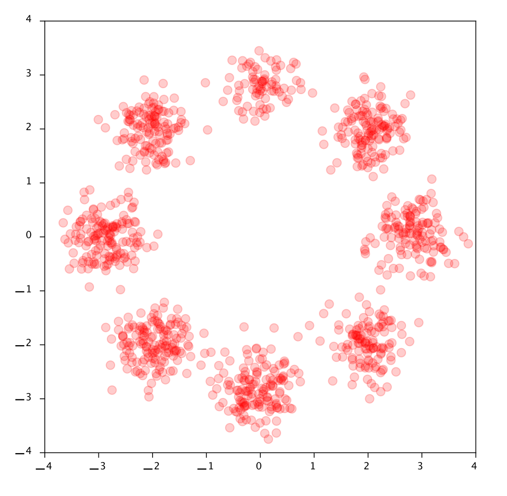
A 1000 datapoints from the 8 Gaussians dataset.
Now we already trained a neural network $\phi$ to do well on this task. You can see in the below image how it transforms the datapoints into the Gaussian base distribution over time:
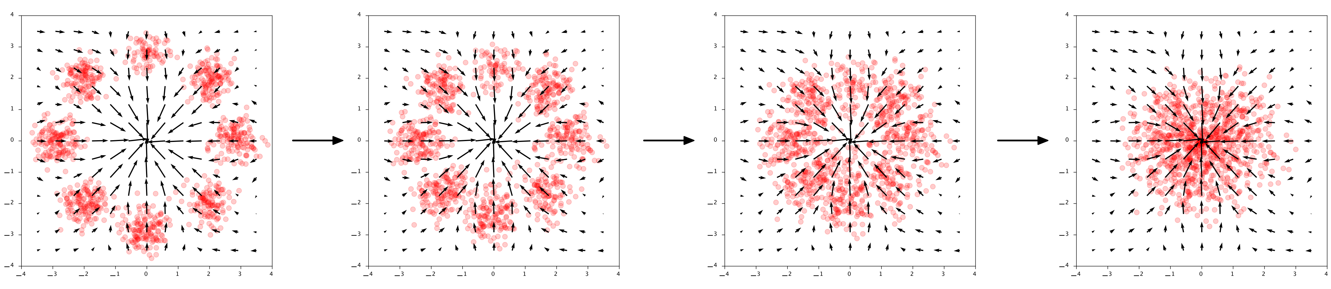
Given data $\mathbf{x}$ transform to $\mathbf{z} = \mathbf{x} + \int_0^1 \phi(\mathbf{x}(t)) dt$. The arrows show the output of $\phi$
The arrow directions in the plots really show the output of $\phi$ at those points. $\phi$ is literally describing how to points should move through the space. Interestingly, for generation we go in the opposite direction, so $-\phi$. To generate points, first we sample Gaussian noise in $\mathbf{z} \sim \mathcal{N}(0, 1)$ and then compute the reverse of the flow:
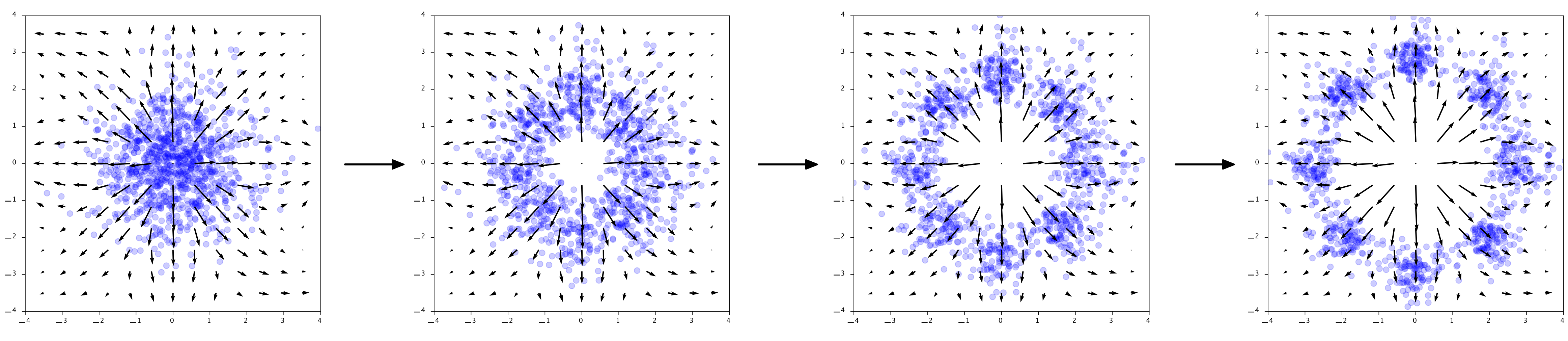
Given noise $\mathbf{z}$ generate $\mathbf{x} = \mathbf{z} + \int_1^0 \phi(\mathbf{x}(t)) dt$. The arrows show the output of $-\phi$
That’s it for continuous-time flows. They are ODEs and have their own continuous time change-of-variables formula that itself is also an ODE.
Some remarks Several details have not been explained. How to compute the gradient efficiently? (Adjoint method). How to compute the trace efficiently? (Hutchinson’s trace estimator). For these details please see the paper by Chen et al. (2018) and Grathwohl et al. (2018). Also $\phi$ may depend on time, but in both notation and visualization it was easier to ignore this.
3. E(n) Equivariant GNNs
Main takeaway Equivariance is about the very intuitive concept of symmetry: If my input rotates, my output needs to rotate similarly. In our work, we are interested in rotations, reflections and translations, which is linked to the Euclidean Group E(n). Therefore, we want a network $\phi$ that is E(n) equivariant. For this we use EGNNs, which are computationally cheap and expressive.
Then the flow $f$ constructed from $\phi$ is also equivariant. And then with this equivariant flow $f$ an invariant distribution $p_X$ can be constructed. This distribution has the desirably property that no matter how you rotate your input, it will give the same likelihood.
E-GNNs, the network $\phi$ is equivariant to rotations and translations.
Equivariance Background Group Equivariant Networks (Cohen & Welling 2016, Dieleman et al. 2016) hard-code symmetries in their transformations. Taking rotations with a matrix $\mathbf{Q}$ as an example: Rotating the input should also rotate the output of a function. Or concisely, $\phi$ is rotation equivariant if: $$\phi(\mathbf{Q}\mathbf{x}) = \mathbf{Q}\phi(\mathbf{x}) \quad \text{ for all rotation matrices } \quad \mathbf{Q}$$
Although the statement might seem technical at first, it’s conveying a very natural constraint that we can all relate to: for some structures it does not matter whether you rotate them or not. And the predictions should be the same, or rotate accordingly.
The Euclidean Group E(n), and how does it act? The group of translations, rotations and reflections is called the Euclidean group, and is referred to as $E(n)$ for short. An element of this group can be described by an $n \times n$ orthogonal matrix $\mathbf{Q}$ and translation vector $\mathbf{t} \in \mathbb{R}^n$. The group is not the full story though, one has to decide how the group acts on the data. Here you want to make choices that fit nature, and although it seems technical it is something that everybody intuitively already understands. Imagine a graph with points that have coordinates $\mathbf{x}$ and a temperature $\mathbf{h}$. Then a rotation and translation act on $\mathbf{x}$ by rotating and translating it, but the same act on the temperature $\mathbf{h}$ will not change it. For this reason we sometimes refer to features $\mathbf{h}$ as invariant. There is a third type of data: velocities $\mathbf{v}$. Although these will rotate like positions, they will not translate. To extend our equivariant notation from earlier, we say $\phi$ is E(n) equivariant if:
$$\phi(\mathbf{Q}\mathbf{x}, \mathbf{h}) = \mathbf{Q}\mathbf{z}_x, \mathbf{z}_h \quad \text{where} \quad \mathbf{z}_x, \mathbf{z}_h = \phi(\mathbf{x}, \mathbf{h})$$
There is a large body of work dedicated to finding expressive networks equivariant to Euclidean symmetries, for example Tensor Field Networks (Thomas et al. 2018).
E-GNNs In E-GNNs (Satorras et al. 2021) we aim to simplify E(n) Equivariant transformations as much as possible, while retaining or improving the performance. The main take-away is the following: Most of the complexity of the transformation is learned via the edge function $\phi_e$ the position function $\phi_x$ and $\phi_h$. Because all these functions operate on an invariant representation, they can be any arbitrary function. To see the invariance: Just imagine rotating the $\mathbf{x}$’s, these functions will not change, because distances $|\mathbf{x}_{i}^{l}-\mathbf{x}_{j}^{l}|^{2}$ do not change under rotations. $$\mathbf{m}_{ij} =\phi_{e}\left(\mathbf{h}_{i}^{l}, \mathbf{h}_{j}^{l},\left|\mathbf{x}_{i}^{l}-\mathbf{x}_{j}^{l}\right|^{2}\right) \quad \text{ and }\quad \mathbf{m}_{i} = \sum_{j \not= i} e_{ij}\mathbf{m}_{ij}, $$
for the messages. The positions and invariant features are updated using:
$$\mathbf{x}_{i}^{l+1} =\mathbf{x}_{i}^{l}+\sum_{j \neq i} \frac{(\mathbf{x}_{i}^{l}-\mathbf{x}_{j}^{l})}{|\mathbf{x}_{i}^{l}-\mathbf{x}_{j}^{l}| + 1} \phi_{x}\left(\mathbf{m}_{ij}\right) \quad \text{ and }\quad \mathbf{h}_{i}^{l+1} =\phi_{h}\left(\mathbf{h}_{i}^l, \mathbf{m}_{i} \right)$$
Together these layers define a single layer. We can just stack them to get a deeper E-GNN. Note that in the update equation for $\mathbf{x}$ we show the more stable version which we introduced in E(n) Flows, which was important to improve the stability of the ODE.
Invariant Distributions with Equivariant Flows In the end we want the likelihood of a point cloud to remain the same under rotations. So we desire: $$p_X(\mathbf{x}) = p_X(\mathbf{Q}\mathbf{x}) \quad \text{ for all orthogonal matrices } \quad \mathbf{Q}$$
Köhler et al. (2019) showed a really cool result: Take an equivariant flow $f$ with an invariant base distribution $p_Z$ with $p_Z(\mathbf{z}) = p_Z(\mathbf{Qz})$. Then together they give a complicated but invariant likelihood $p_X$. In an equation this can be seen from:
$$p_X(\mathbf{Q}\mathbf{x}) = p_Z(f(\mathbf{Q}\mathbf{x})) |\det J_f(\mathbf{Q}\mathbf{x}))| = p_Z(\mathbf{Q}f(\mathbf{x})) |\det \mathbf{Q} J_f(\mathbf{x}))| = p_Z(f(\mathbf{x})) |\det J_f(\mathbf{x}))| $$
You might ask why not take an invariant flow? So something with $f(\mathbf{Qx}) = f(\mathbf{x})$? Then you would also have an invariant distribution $p_X$. Good thinking! However, it turns out that in that case the transformations that you can learn are very limited, and as a result you cannot really model complicated invariant distributions with $p_X$. A final remark: In this section we only talked about rotations, for translations the story is slightly different and for details please see the paper.
4. Argmax Flows
Main takeaway We have a problem, we have a continuous-time flow, which models continuous distributions. However, some features are discrete, like for instance an atom type (Carbon, Hydrogen, Oxygen, …). To lift these discrete values, we use Argmax Flows. Argmax Flows give a way to transition between the categorical and continuous. To discretize we can simply take the argmax: $\mathbf{h} = \mathrm{argmax}\,\,\boldsymbol{\tilde{h}}$. To lift to the continuous, we sample $\boldsymbol{\tilde{h}} \sim q(\cdot | \mathbf{h})$. To optimize, we only need to subtract $\log q(\boldsymbol{\tilde{h}} | \mathbf{h})$ from the objective, and then we are guaranteed to learn a lowerbound on our discrete log-likelihood.
Argmax Flows
First of all, in case of ordinal data (integers like a temperature), Variational Dequantization by by Ho et al. (2019) is exactly what you want. In this section we will focus on categorical data. In the case, we can use Argmax Flows (Hoogeboom et al. 2021). These work as follows: Assume a continuously distributed variable $p(\boldsymbol{\tilde{h}})$ and let $\mathbf{h} = \mathrm{argmax}\,\,\boldsymbol{\tilde{h}}$. For $K$ classes we have $\boldsymbol{\tilde{h}} \in \mathbb{R}^K$ and $\mathbf{h} \in \{0, 1, \ldots, K\}$. This construction gives us a generative model that outputs classes in $\{0, 1, \ldots, K\}$
Now observe the following: we can see the deterministic argmax as a discrete distribution with 100% of the mass on that output. So we say $P(\mathbf{h} | \boldsymbol{\tilde{h}}) = 1\,$ if $\,\mathbf{h} = \mathrm{argmax} \,\,\boldsymbol{\tilde{h}}\,$ and $\,P(\mathbf{h} | \boldsymbol{\tilde{h}}) = 0$ otherwise. This is cool, because sampling from this distribution is exactly the same as taking the argmax.
We can now write the entire thing as a latent variable model and derive for a discrete distribution we define: $p(\mathbf{h}) = \int P(\mathbf{h} | \boldsymbol{\tilde{h}}) p(\boldsymbol{\tilde{h}}) \mathrm{d}\boldsymbol{\tilde{h}}$. Although this integral may seem complicated, it’s just counting for a class $\mathbf{h}$ how much probability mass is in the corresponding continuous region. We then derive in log-space using variational inference: $$ \log p(\mathbf{h}) = \log \int P(\mathbf{h} | \boldsymbol{\tilde{h}}) p(\boldsymbol{\tilde{h}}) \mathrm{d}\boldsymbol{\tilde{h}} \quad \text{from definition}$$
$$ =\log \int \frac{q(\boldsymbol{\tilde{h}} | \mathbf{h})}{q(\boldsymbol{\tilde{h}} | \mathbf{h})} P(\mathbf{h} | \boldsymbol{\tilde{h}}) p(\boldsymbol{\tilde{h}}) \mathrm{d}\boldsymbol{\tilde{h}} \quad \text{multiply by 1}$$
$$ =\log \mathbb{E}_{\boldsymbol{\tilde{h}} \sim q(\cdot | \mathbf{h})} \frac{P(\mathbf{h} | \boldsymbol{\tilde{h}}) p(\boldsymbol{\tilde{h}})}{q(\boldsymbol{\tilde{h}} | \mathbf{h})} \quad \text{integral to expectation}$$
$$ \geq \mathbb{E}_{\boldsymbol{\tilde{h}} \sim q(\cdot | \mathbf{h})} \log \frac{P(\mathbf{h} | \boldsymbol{\tilde{h}}) p(\boldsymbol{\tilde{h}})}{q(\boldsymbol{\tilde{h}} | \mathbf{h})} \quad \text{Jensen’s inequality}$$
For this last step, restrict $q(\boldsymbol{\tilde{h}} | \mathbf{h})$ to only have support over the relevant region: the region where $P(\mathbf{h} | \boldsymbol{\tilde{h}}) = 1$. Then we get
$$ \log p(\mathbf{h}) \geq \mathbb{E}_{\boldsymbol{\tilde{h}} \sim q(\cdot | \mathbf{h})} [\log p(\boldsymbol{\tilde{h}}) - \log q(\boldsymbol{\tilde{h}} | \mathbf{h})] \quad \text{restrict $q$, expand log}$$ And this is exactly the objective that we optimize. What’s cool is that this gives us a very nice method to transition between the categorical space $\mathbf{h}$ and the continuous space $\boldsymbol{\tilde{h}}$ using an argmax function in one direction, and sampling from $q$ in the other direction. The only thing we have to take into account is the additional term $- \log q(\boldsymbol{\tilde{h}})$. Now we are completely free to train any continuous distribution (such as a continuous-time flow) for $p(\boldsymbol{\tilde{h}})$. This is great because $\mathbf{x}$ was already continuous, so to optimize a flow on both positions and features $(\mathbf{x}, \mathbf{h})$ jointly we needed to lift the features $\mathbf{h}$ to the continuous $\boldsymbol{\tilde{h}}$. We then train on $(\mathbf{x}, \boldsymbol{\tilde{h}})$.
Because we can now transition between discrete and continuous so easily, in remaining sections we may not properly distinguish between $\mathbf{h}$ and $\boldsymbol{\tilde{h}}$ anymore. Also sometimes we drop the tilde as in the paper so $\boldsymbol{\tilde{h}} = \boldsymbol{h}$.
How to construct q? This section is not super important, but just for the interested reader. We will give the simplest method we came up with. Recall that we need to sample values $\boldsymbol{\tilde{h}}$ but only in the region where $\mathbf{h} = \mathrm{argmax} \,\,\boldsymbol{\tilde{h}}$, where $\mathbf{h}$ is given as a datapoint. First construct a distribution with free noise $\boldsymbol{u}$, in our case we’ll use a Gaussian $\boldsymbol{u} \sim \mathcal{N}(\mu(\mathbf{h}), \sigma(\mathbf{h}))$, where $\mu, \sigma$ are functions modelled by a (shared) EGNN. Then call $i = \mathbf{h}$ to clarify that it’s an index. We leave the $i$‘th index the same so that $\boldsymbol{\tilde{h}}_i = \boldsymbol{u}_i$. Call this value $T = \boldsymbol{\tilde{h}}_i$. Then all the other indices are thresholded using $\boldsymbol{\tilde{h}}_{-i} = T - \mathrm{softplus}(T - \boldsymbol{u}_{-i}))$, which ensures they are smaller than $T$. So this is exactly the desired argmax constraint. Since the function is bijective, we can use the change-of-variables formula again to find:
$$\log q(\boldsymbol{\tilde{h}} | \mathbf{h}) = \log \mathcal{N}(\boldsymbol{u} | \mu(\mathbf{h}), \sigma(\mathbf{h})) - \log |\det \mathrm{d}\boldsymbol{\tilde{h}}/\mathrm{d}\boldsymbol{u}|,$$
using the derivatives of the softplus. And this is exactly the additional term $\log q(\boldsymbol{\tilde{h}} | \mathbf{h})$ that we need in the objective so we are done :).
5. E(n) Equivariant Flows
Wow, you made it. And there is good news: we’ve been setting up all the relevant parts above so that it fits perfectly for E(n) Equivariant Flows. So most of the hard work is done. First as a reward, let’s look at the generation of a molecule using the E-NF:
Animation of E(n) Flows.
The animation is showcasing two properties of our model. 1) The flow is invertible. This is shown via the generate and inference animations. 2) The flow is equivariant. If not, after rotating we wouldn’t necessarily arrive at the same molecule (but rotated). Only because the model is both invertible and equivariant, we are able to loop this gif.
The Normalizing Flow So what do we need? A description for the positions of the nodes: $\mathbf{x} \in \mathbb{R}^{M \times n}$. So there $M$ nodes in a $n$-dimensional space. Also we need something for features on the nodes, like an atom type, which we call $\mathbf{h} \in \mathbb{R}^{M \times \mathrm{nf}}$, which can contain $\mathrm{nf}$ features. We know now that if $\mathbf{h}$ is categorical, then we can lift them to a continuous version using Argmax Flows. Here $f$ maps $\mathbf{x}, \mathbf{h} \mapsto \mathbf{z}_{x}, \mathbf{z}_{h}$. Then, we join everything together into a change of variables formula:
$$p(\mathbf{x}, \mathbf{h}) = p_Z(\mathbf{z}_{x}, \mathbf{z}_{h}) | \det J_f |,$$
where $J_f = \frac{\mathrm{d}(\mathbf{x}, \mathbf{h})}{\mathrm{d}(\mathbf{z}_{x}, \mathbf{z}_{h})}$ is the Jacobian, where all tensors are vectorized for the Jacobian computation. To build $f$, we utilize an ODE with an E-GNN $\phi$ that is the actual learnable part of our model:
$$\mathbf{z}_x, \mathbf{z}_h = f(\mathbf{x}, \mathbf{h}) = [\mathbf{x}, \mathbf{h}] + \int_{0}^{1} \phi(\mathbf{x}(t), \mathbf{h}(t))\mathrm{d}t.$$
As mentioned before, the solution to this integral is simply solved by calling z = odeint(self.phi, x, [0, 1]). In the next section we can describe the dynamics $\phi$.
Imagine how cool these dynamics are by the way: Previously in the 2D example $\phi$ was only predicting the velocity for 2D points independently. Now it’s way cooler: It’s predicting for a collection of points (for instance a molecule with atoms) how each atom should move depending on all the others. If you look at the visualization, $\phi$ is really deciding how each atom travels through the space.
The Dynamics Using the construction of the EGNN layer in the previous section, we can just stack them to get an EGNN. In the experiments we used 6 layers, so $L=6$. The invariant output $\mathbf{h}^L$ can be used immediately, we denote this $\mathbf{h}^L(t)$ with $(t)$ just because the input depends on a specific time $t \in [0, 1]$. A problem would arise if you used $\mathbf{x}^L(t)$ immediately: the ODE would not be equivariant anymore. Instead, we need the dynamics for $\mathbf{x}$ to behave like a velocity vector: It should rotate, but not translate under the group actions. The reason for this is that $\mathbf{x}$ itself already translates under group actions, so just adding the output $\mathbf{x}^L(t)$ would double that action, essentially translating the output twice. This is easily alleviated by using the residual $\mathbf{x}^L(t) - \mathbf{x}(t)$, which does behave as a velocity. We can then write the dynamics of our model, the main learnable component as follows:
$$\phi(\mathbf{x}(t), \mathbf{h}(t)) = \mathbf{x}^L(t) - \mathbf{x}(t), \mathbf{h}^L(t) \quad \text{ where } \quad \mathbf{x}^L(t), \mathbf{h}^L(t) =\text{EGNN}[\mathbf{x}(t), \mathbf{h}(t)].$$
And that’s it. We now have a model that can be trained on molecule-like data.
Samples Training takes about a week or two. Continuous-time normalizing flows are just really expensive, requiring hundreds of evaluations to solve the ODE. Nevertheless, the results are really awesome. We show our method far outperforms existing normalizing flow methods on several datasets. Among these is qm9 which contains molecules, and from that model we can show these samples we generated:
Samples from the E(n) Flow trained on qm9.
An overview
And then the overview of what we actually do during training. The flowchart below shows the steps:
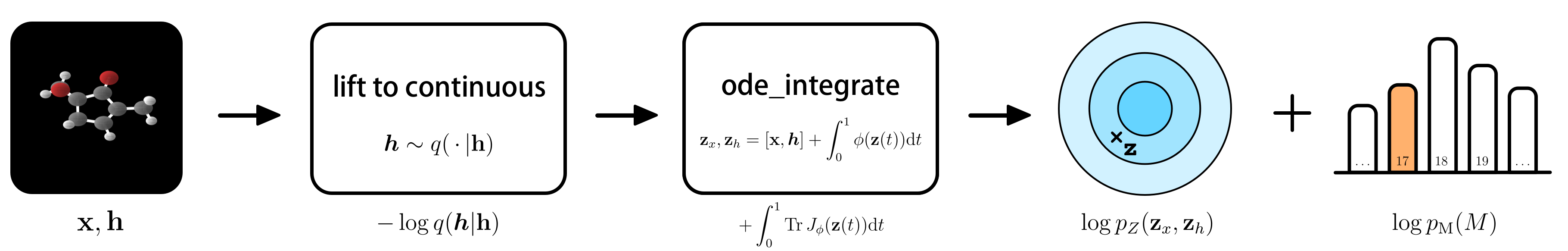
Training E(n) Equivariant Flows
odeint using the dynamics $\phi$ modelled by an EGNN. 3) Collect all the terms for the likelihood among which is the base distribution on the output: $\log p_Z(\mathbf{z}_x, \mathbf{z}_h)$. To deal with different molecule sizes, an addition 1D categorical distribution $p(M)$ (think of a histogram) models the molecule size. At last, we can show the objective in its entirety, which brings everything together in a single line:
$$\log p(\mathbf{x}, \mathbf{h}) \! \geq \! \mathbb{E}_{\boldsymbol{\tilde{h}} \sim q(\cdot | \mathbf{x}, \mathbf{h})} [\underbrace{\log p_Z(\mathbf{z}_x, \mathbf{z}_h)}_{\text{base likelihood}} + \underbrace{\int_0^1 \mathrm{Tr }\, J_{\phi}(\mathbf{x}(t), \boldsymbol{\tilde{h}}(t))dt}_{\text{ODE volume change}} \, \underbrace{-\log q(\boldsymbol{\tilde{h}} | \mathbf{x}, \mathbf{h})}_{\text{lifting term}} + \underbrace{\log p(M)}_{\text{size likelihood}}],$$
where $\mathbf{z}_x, \mathbf{z}_h = [\mathbf{x}, \mathbf{h}] + \int_{0}^{1} \phi(\mathbf{x}(t), \mathbf{h}(t))\mathrm{d}t$.
Conclusions
And that’s it. In spite of the good results there are some limitations: 1) Continuous-time flows are computationally expensive. 2) The combination of the ODE with the original EGNN is sometimes unstable. After our modification, we still noticed some rare peaks in the loss of the QM9 experiment that can diverge. (Of course when the model is saved you can simply restart from right before that point in training). 3) The model in its current form does not model distributions over edges between nodes. 4) Our likelihood estimation is invariant to reflections, but some structures (like molecules) may be chiral: their mirror image does not interact in the same way as the original. Also, if you are specifically interested in molecule generation also have a look at the work by Gebauer et al. (2019). And that’s it, thank you for reading :).
References (in order of appearance)
Victor Garcia Satorras, Emiel Hoogeboom, Fabian B. Fuchs, Ingmar Posner, Max Welling. E(n) Equivariant Normalizing Flows. (2021)
Danilo Jimenez Rezende, Shakir Mohamed. Variational Inference with Normalizing Flows. (2015).
Laurent Dinh, Jascha Sohl-Dickstein, Samy Bengio. Density estimation using Real NVP. (2016)
Changyou Chen, Chunyuan Li, Liqun Chen, Wenlin Wang, Yunchen Pu, Lawrence Carin. Continuous-Time Flows for Efficient Inference and Density Estimation (2017)
Ricky T. Q. Chen, Yulia Rubanova, Jesse Bettencourt, David Duvenaud. Neural Ordinary Differential Equations. (2018)
Will Grathwohl, Ricky T. Q. Chen, Jesse Bettencourt, Ilya Sutskever, David Duvenaud. FFJORD: Free-form Continuous Dynamics for Scalable Reversible Generative Models (2018)
Taco Cohen, Max Welling. Group Equivariant Convolutional Networks. (2016)
Sander Dieleman, Jeffrey De Fauw, Koray Kavukcuoglu. Exploiting Cyclic Symmetry in Convolutional Neural Networks. (2016)
Nathaniel Thomas, Tess Smidt, Steven Kearnes, Lusann Yang, Li Li, Kai Kohlhoff, Patrick Riley. Tensor field networks: Rotation- and translation-equivariant neural networks for 3D point clouds. (2018)
Victor Garcia Satorras, Emiel Hoogeboom, Max Welling. E(n) Equivariant Graph Neural Networks. (2021)
Jonas Köhler, Leon Klein, Frank Noé. Equivariant flows: sampling configurations for multi-body systems with symmetric energies. (2019)
Jonathan Ho, Xi Chen, Aravind Srinivas, Yan Duan, Pieter Abbeel. Flow++: Improving Flow-Based Generative Models with Variational Dequantization and Architecture Design. (2019)
Emiel Hoogeboom, Didrik Nielsen, Priyank Jaini, Patrick Forré, Max Welling. Argmax Flows and Multinomial Diffusion: Learning Categorical Distributions. (2021)
Niklas W. A. Gebauer, Michael Gastegger, Kristof T. Schütt. Symmetry-adapted generation of 3d point sets for the targeted discovery of molecules. (2019)
This list is by no means comprehensive, check out the paper for more details.